Older Method for Automatic Assignment and Fitting - The ν11
band of cis-1,2 Dichloroethene
Note: This page has been superseded for
this particular spectrum by a method including the nearest lines
window - see Automatic Fitting of the nu5
band of cis 1,2-Dichloroethene. It has been left in
the documentation because it is a legitimate way of working where
the aim is to match small sections of a spectrum.
This page provides a detailed walk through to
accompany "Automatic Assignment and Fitting of Spectra with PGOPHER".
C. M. Western and B. E. Billinghurst, Physical Chemistry Chemical
Physics, 19, 10222 - 10226 (2017), doi:10.1039/c7cp00266a.
It describes the process of assigning and fitting a high
resolution (0.001 cm−1) spectrum of the ν11
band of cis-1,2-dichloroethene at 570 cm−1, taken
at the Canadian Light Source. It assumes some familiarity with the
basic operation of PGOPHER, as in Walk-through
of Simulating and Fitting a Simple Spectrum. The raw
initial spectrum is provided as nu11raw.ovr; this
essentially as saved by the spectrometer, but with the only region
around the ν11 band saved.
A. Converting to a line list
The first step is to convert the spectrum to a list of line
positions and intensities. This can be done with an external tool
if required, but the internal tool is described here.
- Load original spectrum, nu11raw.ovr.
-
Right click on the overlay and select "Baseline...".
This brings up a window allowing a baseline algorithm to be
chosen, and then an automatic peak finder to be run. Tools for
zooming and panning are available at the top of the window,
and work in the same way as those on the main window.
-
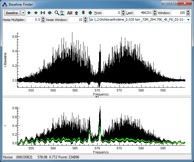
Press the "Baseline" button to calculate a
baseline. The orange line shows the calculated baseline, and
the green line indicates the upper limit of the points used in
calculating the baseline. This spectrum clearly has a ripple
in it; setting "Window" non-zero turns on a algorithm
involving a moving average over the specified window to
identify the baseline. It works by attempting to identify
points on the baseline (within the "Noise Multiplier");
for this spectrum turning on the "Dense" option in
the drop down menu, found by clicking on the small down arrow
by the "Baseline" button helps. Try 100 for the "Window"
and 0.5 for the "Noise Multiplier". Pressing
"Baseline" should yield a display like this:
The baseline around the band heads is not right, but these are
too dense for simple assignment anyway.
-
If you want to save the spectrum with the
baseline subtracted, select "Apply to New" from the drop down
menu to generate an overlay as shown in the upper trace,
though this is not necessary in this case.
-
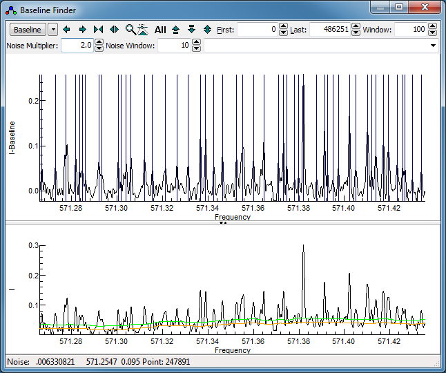
To try the line finding algorithm, zoom in
on a small region so that individual lines are clearly
visible. Turning on "
Live update" from the drop down
menu (next to the "
Baseline" button) will show the
lines found in the upper window in blue automatically as the
parameters are changed. (Note this can be slow if the selected
region is large.) Adjust the "
Noise Multiplier" to
give a sensible set of peaks indicated in the top trace. It is
not necessarily the same as used for the baseline calculation
- in this case a "
Noise Multiplier" of 2 is
promising, giving a display something like this:
-
From the drop down menu, select "Make
Linelist". This will generate a line list that shows in
the main window.
-
The resulting line list is saved as
nu11line.ovr. To
save space the raw spectrum has been deleted, though for the
later steps it can be helpful to have both spectra available,
and peaks missed by the automatic peak finder can be measured
manually if needed. (To load two overlays at once drag and
drop both files onto the main window, or use "
File, Load
Overlay..." followed by "
File, Add Overlay...".
B. C2H235Cl2
1. Rough Alignment.
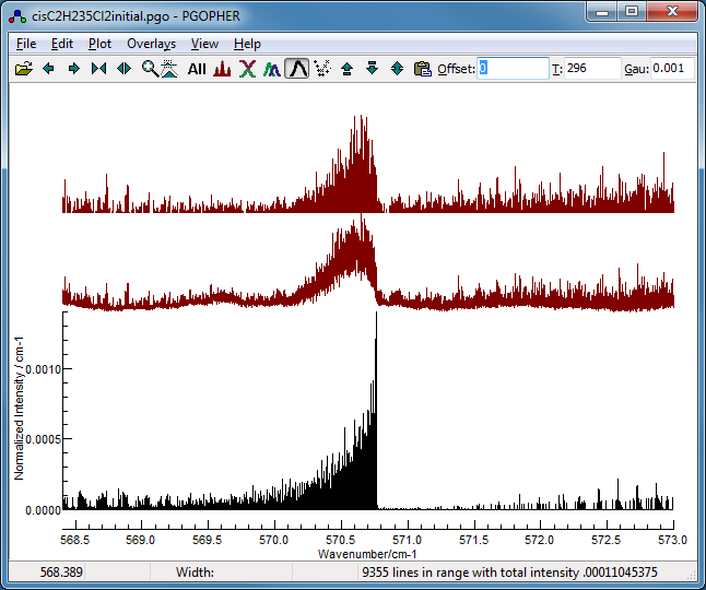
The obvious starting point is with the most abundant species. An
initial simulation is provided in cisC2H235Cl2initial.pgo. This
is a standard asymmetric top simulation set up as follows:
- Constants for both states were initially set to those
determined by a microwave spectrum of the ground state (Leal et
al, 1994).
-
As this is a near prolate top, the upper
state parameters were converted to use Bbar
= ½(B+C) and δ = B−C,
as the spectrum is relatively insensitive to the latter.
-
Some manual adjustments to the
Origin, and Bbar were made to obtain a
spectrum that was roughly right by comparing to a low
resolution spectrum from the PNNL database (Sharpe et al,
2004).
-
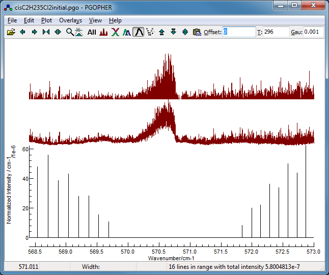
The simulation suggests the region around
the 35Cl2 band head, excluding the 35Cl37Cl
band head is likely to be dominated by the 35Cl2
species, so this is used as the starting point for the fit:
2. Initial search for Ka = 6 lines
Looking for Ka = 6 lines is a
good starting point as higher K values typically behave
very close to a symmetric top, so the spectrum is unlikely to be
sensitive to δ. In addition the lines will all have much the
same contribution from A, so only two parameters, Bbar
and the Origin, will be needed to fit this set of lines.
- For an initial search for Ka = 6 lines open
the transitions window (View,
Transitions) and select:
-
"Change" as "<>", which
hides the Q branch transitions. The Q branch is unlikely to
make a good search target because almost all of the lines
are blends.
- Upper state Ka as 6.
-
Upper state symmetry as O+. This selects
one of the pair of near degenerate Ka = 6
lines, which are not resolved here. (Which of the two is
chosen is not important.)
- Make sure "Filter" is checked and then select:
-
The resulting plot confirms the regular
pattern, much like the classic P and R branch combination of a
linear molecule, which will therefore be described by two
effective parameters:
-
When you are happy with the selection
displayed click "
Add". This will add entries to the
line list window for all the
transitions selected by the transitions window.
-
In the line list window, make sure "More,
Advanced" is selected to make the advanced settings
visible. Set "Accept" to the maximum error you expect
for the "check" transitions - in this case try 0.001,
approximately the line width.
- Bring up the auto fit window with "Overlays", "Autofit..."
-
Set "Window" to the search window
for the initial fits, i.e. how far each side of the initial
line positions you want to search. This should reflect how far
out you think the lines might be - try 0.3 cm−1
here, which is approximately the distance between the selected
lines.
- Select the upper state parameters to float in the constants window. - in this case
Bbar and Origin.
-
Select the lines for the trial assignment
in the
line list window - these
should be lines that you are reasonably confident will be
clear in the spectrum. In this case two lines are enough, and
the P branch region looks clearest. Some separation in
J
is likely to give the best determination of constants, so try
P(11) and P(14) (These appear with their full labels,
qP
6,6(11)
and
qP
6,9(14) respectively). To select
these two lines, click on (say) the P(11) line and use the up
(or down) arrow buttons at the top of the line list window to
move it next to the P(14) line. Then click and drag over the
P(11) and P(14) rows so that both are selected.
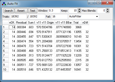
- The file at this stage is saved as cisC2H235Cl2_A.pgo.
-
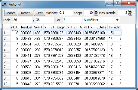
Press "Search" in the Auto Fit
window. There will be a short delay as the search is done.
- When the search is complete, the best fits will be presented
in the auto fit window, which lists:
- nOK - the number of "check" transitions within
the "Accept" window
- Residual - the RMS observed - calculated for
these "check" transitions.
- SumI - the sum of observed intensity for these
"check" transitions.
- The values of the constants obtained for each fit.
- Trial - The number of the trial. (This is
typically only useful for debugging purposes.)
- nDiff - the number of transitions different to
the selected fit. This is only displayed if one of the
fits is selected.
Some additional information is shown in the log window.
-
To try out an individual fit, double click
on that row. This will update the line list window with all
the assignments made by that fit, and display the
residuals window with the
obs-calc plotted for the assignments made. The standard
PGOPHER
fit process can then be used to refine the fit. If you don't
like the result, the "
Reset" button will discard the
new assignments and reset the parameters.
-
In this case none of the fits look
promising, though each fit has a low residual. Inspection of
the results indicates a wide variation in the origin values,
but the location of the origin is pretty clear in the
experimental spectrum. To limit the possible range for
parameter values, set the maximum permitted change (+ or
−) in the "Std Dev" column in the constants
window for the required constant. This will speed up the
search process, as trials can be discarded more quickly. In
this case try a value of 0.1 for the Origin, and try again
from step 9 above. (Make sure you have pressed "Reset"
so that all assignments are removed.)
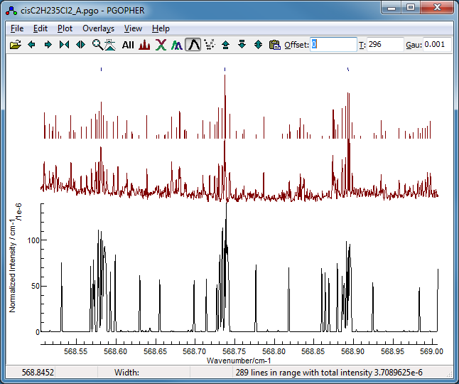
-
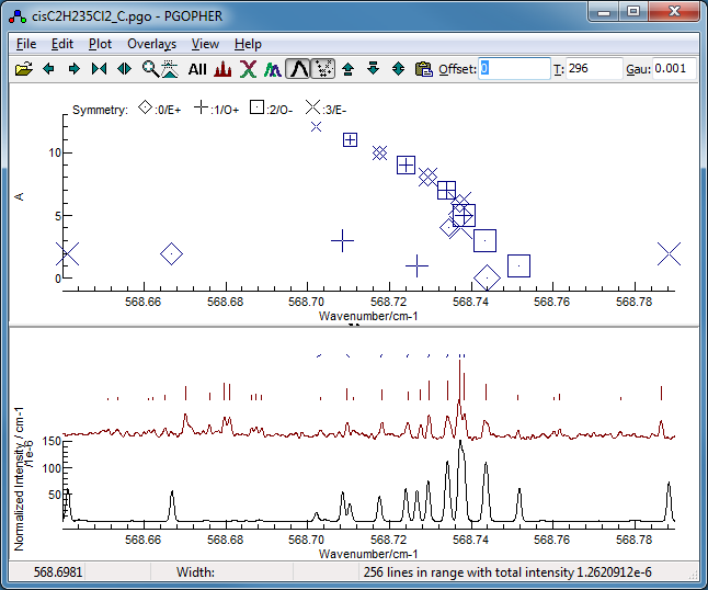
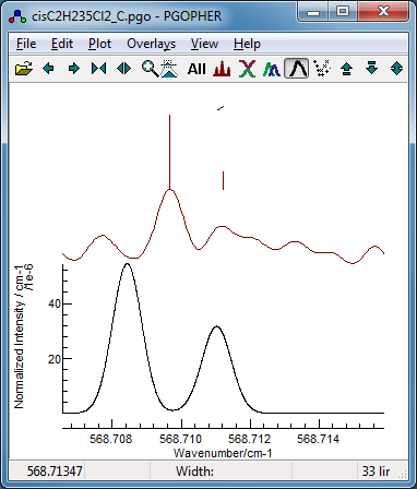
Now fit number 3 looks promising,
especially looking at the region around 568.7 cm
−1:
This shows the
K sub bands with approximately the
right spacing, though the detail is wrong.
-
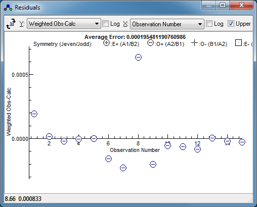
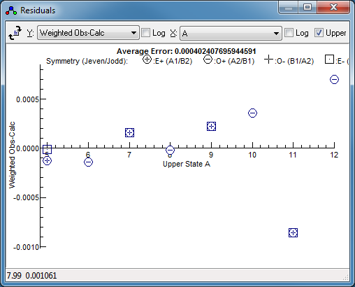
Once you have found an initial fit that
looks good, press fit in the line list window a couple of
times. This will fit all the assigned lines in the normal way,
and produce revised constants. The residuals window can be
very helpful here; for the worked example here it clearly
indicates one transition as much a much worse fit than the
others, so should be checked:
To do this, right click on the point in the observations
window and try one of the following:
-
Select "
Show and Edit". This
will highlight the relevant observation in the line list
window, and centre the plot on the transition. (This is most
useful if the "Expand range" button (

)
is pressed a few times so the window only shows a small plot
range.) Setting the "
Std Dev" for this line to
blank in the line list window will remove it from the fit.
-
The quick fix (... to sweep it under the
carpet) is simply to select "Remove Point(s)". This
will set "Std Dev" to 0 for this transition,
excluding it from the fit.
-
3. Initial fit of the Ka structure of the
P(13) lines
While the K sub-bands are now in
approximately the right place, the structure within them is not
right. The obvious constant to fit next is A, as this
determines the structure within the sub-band. δ = B−C
is also important,but the range of Ka can be
chosen to be insensitive to this. (Note the selection rule for
this band is ΔKa = 0, so selection can be
in the upper or lower state.) To see the Ka
dependence, set up the plot as follows:
-
Turn on the Fortrat plot (Plot, Fortrat,
Show). This adds an extra window, where the vertical
axis is a selected quantum number. For the current case two
changes need to be made to make the plot usable:
-
Low intensity lines need to be ignored
for the purposes of plotting; in the constants window,
select the "Simulation" object and set "MinI"
to 0.1
-
The quantum number plotted defaults to J,
but Ka is more useful. In the same "Simulation"
object, set "FortranQno" to A.
-
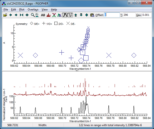
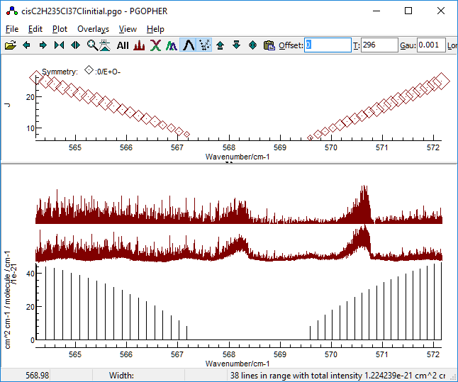
Pressing the simulate button now gives a
plot showing the higher Ka lines are close
together, and show a regular pattern, but the pattern of the
lower Ka lines is much less obvious. The plot below shows the
P(13) region, which looks reasonably clear:
-
Given the lines are all close together, it
is not obvious that the current assignments of Ka
= 6 lines are correct, so it is probably best to remove all
the assignments. Press Clear In the line list window
to do this.
-
The plot above suggests
Ka
≥ 5 lines form a regular pattern, and do not show any
asymmetry splitting at this resolution. As the lower
Ka
lines are stronger, this suggests a search in
A using
Ka = 5 and 6 as fit transitions, with higher
Ka lines as check transitions. To set this
up, open the
transitions window
and, clear any
Ka and symmetry values set,
and set lower
J = 13. "
Change" should
strictly be "
P", though makes no difference in this
case.
-
Hit
Add to add these transitions
to the line list window. To exclude the
Ka
< 5 lines from the fit, delete them from the line list
window. Individual lines can be deleted by clicking on the
line, and then the delete button (the cross

) in
the top row. In this case sorting the lines first (
"More,
Sort On,
Branch" in the linelist window)
can speed things up, as multiple lines can be selected by
clicking and dragging before deleting.
-
To set the search up, select one P5
and one P6 line, using the up and down arrow
buttons if necessary to move them next to each other, and then
clicking and dragging to select the two rows.
-
Some adjustments are also required in the
auto fit window; the search range can be reduced - try "Window"
= 0.03 cm−1. "Max Blends"
needs altering also; this sets the maximum number of
assignments that can be assigned to any one observed line, and
the as the sub-band looks as though is has a band head blends
are likely - try 3 for this, rather than the default of 0.
-
The parameters to float should now be A
and Origin; BBar should be fixed as the
lines selected will not determine this. Floating the Origin
gives a way for the relative position of the sub-band to be
varied. Note that this will have StdDev set, which
will limit the search range; I suggest clearing this, or at
least increasing the value to avoid unreasonably restricting
the search range.
- The file at this stage is available as cisC2H235Cl2_C.pgo.
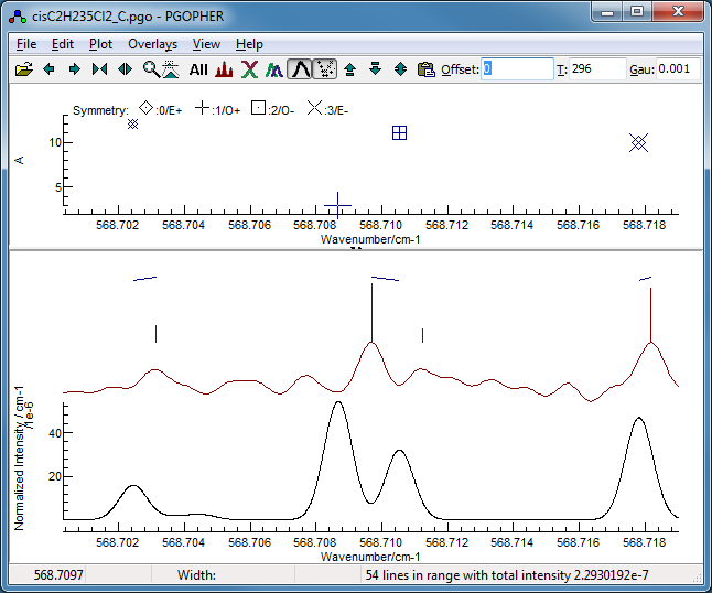
- Press Search; this is now a very quick search, and
the first fit looks very promising:
-
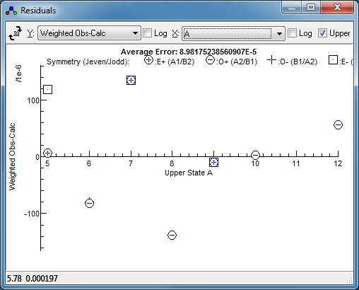
Press fit a couple of times. The
residuals window might not
indicate any problems at first glance, but changing the
horizontal axis to
Ka reveals a systematic
trend. This is selected by setting "
X" to "
A",
which gives:
-
Right clicking on the Ka
=11 mark in this window, selecting "Show and Edit",
and zooming the display a couple of times indicates a possible
reason - perhaps the assignment should have been made to the
weaker peak to higher frequency, rather than the stronger peak
to lower frequency:
-
Approaches to fixing this include manually
making the alternative assignment; right clicking and dragging
on the observed transition will replace the assignment with
the newly measured peak, as the transition will be selected in
the line window. The measurement can be on the original
spectrum (for peaks that were not found in the original line
list generation) on in the line list, where the assignment has
failed. Note that you may have to do this twice, as most lines
are doubled because of the unresolved asymmetry splitting.
-
Alternatively, simply exclude this (pair
of) lines from the fit - right click on the point in the
residuals window, and select Remove Points. Fitting
now gives a much smaller residual (by a factor of 4) and no
obvious trend:
-
To recalculate the positions of the
unassigned lines in the
line list
window, click on "
All" in the line list window
(to select all the lines) and then
"Update", which
will replace the "
Position" column with values
calculated with the current set of constants for transitions
that have not been assigned (i.e. where "
Std Dev" is
blank or zero).
-
With this updated calculated line list, the
"Nearest" button in the linelist window will assign
any unassigned lines to the nearest line in the line list,
provided it is within the acceptance window. In this case it
assigns the Ka = 11 lines to the
alternative peak:
- After a pressing Fit a couple of times, the resulting file is
saved as cisC2H235Cl2_D.pgo.
4. Complete fit of the Ka structure of the
P(13) lines
The next step is to add the Ka < 5 lines
back into the line window, and determine δ = B−C.
To do this:
-
Bring up the
transitions
window - this should still have lower
J = 13 as
above, unless you have changed something. Hitting
"Add"
will add the low
Ka transitions back to the
line list window. Provided "
Discard Duplicates" is
selected, only lines not already present in the line list
window will be added. For all the
Ka
values to be included, you will have to ensure the plot range
is sufficient - if you have zoomed in following the
instructions above zoom out.
-
To set the search up select a single low Ka,
say Ka = 0, and float Origin, A
and BDelta. To avoid limiting the search range,
clear the "Std Dev" column for these parameters. Note
that, as the other assigned lines will be included in the
trial fit, only a single selected line is needed, even though
three parameters are to be determined.
-
Given the large spread of the low Ka
transitions, a slightly larger search window might be required
- try "Window" = 0.1. (The search will in any case be
fast, as only a single line is assigned.)
- The file at this stage is saved as cisC2H235Cl2_E.pgo.
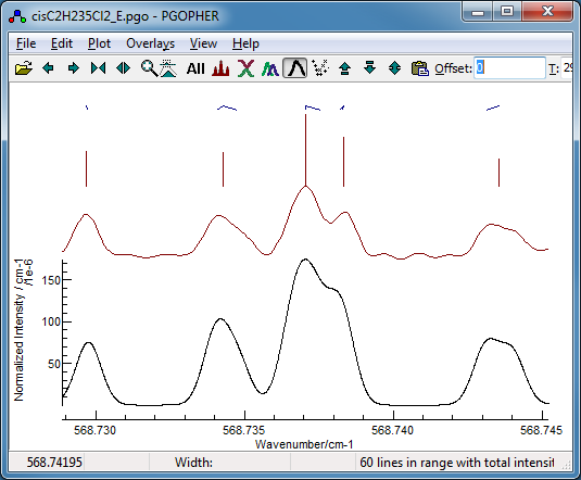
-
Pressing "Search" is again very
quick, and the first two fits are quite promising. Note
that the simulated spectra for the two fits are very similar,
and a useful indicator for this is the nDiff column,
which indicates that these two transitions only have two
transitions with different assignments:
-
Given the similarity, either fit could be
used; the differences are likely to be resolved at a later
stage. Taking the first fit (as it has the lowest residual)
and pressing fit a couple of times gives a good fit with an
average error much less then the linewidth. The
residuals window suggest a
couple of lines have slightly larger errors, and investigation
indicates these are blended lines:
- Removing these for the time being and fitting gives cisC2H235Cl2_F.pgo.
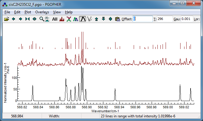
5. Fit of the P(12) lines
The final step is to determine Bbar, which is
straightforward as simulation of the P(12) lines is already quite
good:
- The above plot is generated by using the transitions window to select
transitions with lower state J = 12; note that the
correct range was selected simulating the J = 12
transitions, and then pressing "All" in the
transitions window. This is done automatically if "Plot
All" is checked. Press "Add" to add these to
the line list window, and then set up a search by selecting a
single strong P(12) line, say qP6,6(12).
As in the previous search, the previously assigned lines are
included in the fit, so only a single line is required. The
fitted parameters can now include Origin, A,
Bbar and Bdelta; the "Std Dev" for
these should again be cleared to avoid limiting the range. The
file at this stage is saved as cisC2H235Cl2_G.pgo.
- Pressing search gives a very good fit as the first choice,
and all three upper state rotational constants are now
determined. The above process reassigns the blended lines we
had excluded. These lines can be removed completely or
assigned a larger "Std Dev" in the linelist window;
removing them gives cisC2H235Cl2_H.pgo.
6. Completing the fit
The next step involves adding as many lines as possible to the
fit, which can be done by walking down and up in J. As
many predictions will now be close to the observations, a search
need not be done, and a simple assign to nearest approach can be
used, for example:
- Use the transitions window to add the P(11) lines to the
line list window, and assign them to the nearest line with the
"Nearest" button in the line list window. The
"Nearest" button in the transitions window
performs both these steps and additionally performs a complete
fit cycle, and is particularly useful for walking along a
series of transitions. Either of these assigns all the P(11)
lines, though the residuals window suggests a couple are
slightly off. If you are confident that these are simply
blends, then draw a box round the points you want to keep (as
shown below) then right click and select "Remove Points
Outside".
- This process is easily repeated walking downwards in J;
taking this down to P(5), where the Q branch lines start to
obscure the P branch lines, gives cisC2H235Cl2_I.pgo.
- At this point switching to R branch lines gives an
independent check of the assignments to date. Staring with
R(5) and working upwards in J shows most predicted
peaks matching, though it is less clear here than in the P
branch region because of interference from the 35Cl37Cl
species. Given the high probability of blends, the R branch
lines were not included in the fit.
- The clearest unassigned transitions are now the the P branch
- P(14), P(15) (partially obscured by a Q branch band head),
and then P(19). At P(19) it is worth trying to float the
quartic centrifugal distortion terms. Stepping up to P(30)
gives cisC2H235Cl2_J.pgo.
Stepping up to P(39) gives cisC2H235Cl2_K.pgo;
the sextic centrifugal constants have been floated for this.
There is also some evidence for localised perturbations, with
some transitions being out of place, so we stop at this point.
In publishing the final fit, I recommend including a fit log file
run with "
PrintLevel" set to "
Detail". This
gives a complete set of information about the fit, including the
correlation matrix and matrix elements used, which aids use of the
fit results elsewhere and makes sure the fit can be reproduced.
The "
PrintLevel" setting is found in the top level
object; reset the value to "
Mininal" after producing the
log to avoid slowing the program down by producing unnecessary
output. The final log file is available as
samples/autocis/cisC2H235Cl2.log;
to produce this file the "
Precision" setting (also in the
top level object) was increased from the default value of 4 to 5.
This increases the precision of some of the displayed values in
the log, including the observed and calculated values.
C. C2H235Cl37Cl
The process here is given in outline; refer to the process
above if you need reminding about the details.
1. Rough Alignment.
Assignment for the mixed isotopologue proceeds much as for the
35Cl2 species, with constants for both
states initialized from the ground state microwave spectra (Leal
et al, 1994), with some manual adjustment of the Origin
and Bbar for rough agreement with the observed
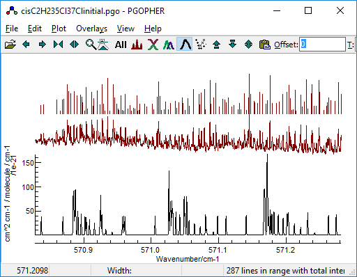
spectrum. This file is available as cisC2H235Cl37Clinitial.pgo.
Identifying a region clear of the 35Cl2
species is tricky, but there is a region immediately to higher
frequency of the 35Cl2 band head that
looks promising, particularly as the 35Cl2
simulation only shows weak lines:
2. Initial fit to A and Bbar
In this case a three parameter search was used, using Ka
= 6 and 7 lines for a range of J values.
-
In the transitions window, select upper
state Ka = 6, symmetry = E+O−, change
"<>". With the aid of the Fortrat plot, adjust the plot
range to select lower state J ≤ 25. The choice of
the range of J is not crucial, but the idea is to give
sufficient intense lines, but to avoid a region where
centrifugal distortion is significant.
-
While these are strong lines, of which a
reasonable number might expect to appear in the fit, the
region around the 35Cl2 band head is
too crowded to give useful assignments, so after pressing "Add"
in the transitions window, manually delete the R branch lines
below 570.8. If there are too many lines in line list window,
check you have the correct filter settings in the transitions
window. The lines in the line list window can be sorted by
frequency (if they are not already sorted) with More,
Sort On, Frequency.
- Repeat the process for to add Ka = 7 lines,
again deleting the R branch lines below 570.8.
-
To set up a search requires three lines to
be identified. Given the region immediately to high frequency
of the 35Cl2 band head is clear, three
R branch lines from this region are an obvious choice. A
possible choice is qR6,10(16),
qR6,11(17) and qR7,11(17);
move these to the top of the line list window with the move to
top arrow button so they are adjacent, and then click and drag
to select these three transitions.
-
To set up the search use acceptance window
of 0.001 cm
−1 (the linewidth) as before and a
search window of 0.3 cm
−1. "
Max Blends"
could be 1 (as the
Ka = 6 and 7 lines for a
given
J could overlap), and limiting the Origin search
range to 0.1 is also required. Float
Origin,
A
and
Bbar. The file at this stage is available as
cisC2H235Cl37Cl_A.pgo.
-
Press
Search - as there are a
large number of possible assignments (6.3 × 10
6)
you will be prompted if you want to continue. The search will
take 5-15 minutes, depending on the speed of your computer.
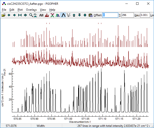
The file after the search (which includes the results of the
search) is available as
cisC2H235Cl37Cl_Aafter.pgo.
-
Trying the results, the first one gives
promising results in the region we have identified as clear:
The others are all much worse, which might suggest using a
search with a restricted search range on all of the parameters
might be required to give more candidate fits.
3. Fitting A, Bbar and δ
-
Taking the first fit - press "
Fit"
to give the best values - we can proceed as for the main
isotopologue, as we have essentially reached step 4. All the
J"
= 17 lines look reasonably close, suggesting a search on these
for
Origin, A and
Bdelta with
three lines selected. I suggest deleting all the previous
assignments at this stage to allow for some minor
re-assignments, and adding all
J" = 17 lines to the
line window for fitting to. The search saved in
cisC2H235Cl37Cl_B.pgo
has
qR
0,17(17),
qR
6,12(17)
and
qR
13,5(17) selected, "
Max
Blends" = 3 and a search window of 0.1 cm
−1.
This range is probably rather wider than needed at this stage,
but it is nevertheless reasonably fast. (Interestingly, using
qR
5,13(17) as one of the selected lines
does not give good results, and subsequent work suggests some
Ka = 5 lines are perturbed.)
-
Fit number 1 is clearly the best and
adjusting the fit using with the help of the residual plot
yields a good fit to all the lines, available in
cisC2H235Cl37Cl_C.pgo.
(The
qR
5,13(17) is clearly slightly out
of position based on this simulation; the intensities indicate
it is not simply a blend. The other two lines excluded from
this fit are simply blends.)
-
Moving on to the R(18) sub-band we can now
determine all 3 rotational constants with a quick search based
on just one line, say
qR
6,13(18).
Clearing the search ranges for all the parameters gives
cisC2H235Cl37Cl_D.pgo
and the search is now very quick, and the first fit is clearly
better than any of the others.
-
Moving on to R(16) the fit is confirmed,
and the
Nearest button in the transitions window can
be used to add and fit these lines, though the plot range
should be reduced to exclude the band head region. R(15) can
similarly be added. After some tidying up,
cisC2H235Cl37Cl_E.pgo
results.
-
Switching to the P branch region is a
possible path at this point, as it is not possible to go to
lower
J in the R branch. While there is more
interference from the main isotopologue, P(15) has sufficient
lines showing for assignment. Assigning this, and stepping
doen to P(8) yields good results (
cisC2H235Cl37Cl_F.pgo),
though a significant number of lines have been excluded as
blends.
-
At this stage the R branch transitions seem
clearer, so try stepping upwards starting at R(19). Consider
starting to float the centrifugal distortion parameters; in
this case try floating these when R(22) is reached. It is then
possible to walk the assignment up to R(30) fairly easily, at
which point the strength and number of the
35Cl
2
lines becomes a concern. A bit of editing is required at each
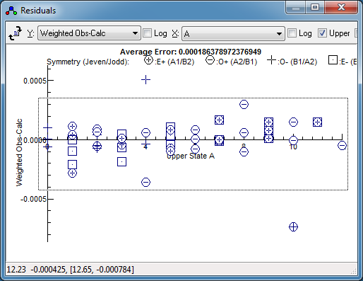
J to check on the larger residuals. Keeping the
largest individual error to around 0.00045 cm
−1 gives
a fit with an average error of 0.00017 cm
−1,
available in
cisC2H235Cl37Cl_G.pgo.
The log file for the final fit is available as samples/autocis/cisC2H235Cl37Cl.log.
References.
- L. A. Leal, J. L. Alonso and A. G. Lesarri, J. Molec.
Spectrosc., 165 368-376 (1994).
- S. W. Sharpe, T. J. Johnson, R. L. Sams, P. M. Chu, G. C.
Rhoderick and P. A. Johnson, Appl. Spectrosc., 58,
1452-1461 (2004).
 Procedures Automatic Fitting