Procedures

<Prev Next>

Contour Fitting

1. To start a contour fit, Overlay the experimental spectrum over the PGOPHER simulation. The initial match must be quite good for a contour fit to work - a contour fit will typically not move a peak more than the peak width, for example.
2. The simulation must also account for all the significant features in the spectrum; if, for example, there are nearby bands that you have not included you should remove the appropriate frequency range from the experimental data. To select part of the experimental spectrum, adjust the plotted range to just cover the range you want to fit, and then right click on the experimental spectrum and select "Select Visible". (If this menu entry is not visible when right clicking, click on the plot style button () until the required spectrum is displayed separately from other plots.) This will restrict plotting and fitting to the selected range; to reverse the process right click and use "Select All". Alternatively, the Crop command described in the  Experimental Overlay section may help with this.
3. It is easier to work if the intensity units of both the overall overlay, and the specific overlay(s) to be floated are set to "Normalised", rather than arbitrary. Go to the overlays window (View, Overlays), click on the topmost item and ensure that "IntensityUnits" are set to "Normalized". Click on the specific overlay and check the same setting. After doing this the "Baseline" and "Scale" will typically need to be adjusted manually for a reasonable match with the simulated spectra as the vertical autoscaling is now turned off.
4. Open the constants window (View, Constants) and click on "Fix", "Fix All Parameters" and select "Mixture"  to ensure that no molecular constants are floated to start with.
5. The first parameters to be floated must be the scale and baseline of the overlaid spectrum. Go to the overlays window (View, Overlays), select the overlay required (probably the first one unless you have more than one experimental spectrum overlaid) and float these two parameters (click in the float column so it reads “yes”).
6. (Optional step) If the required "Scale" is several orders of magnitude different from one, consider scaling the original data to avoid problems with the fitting process later. "Operate", "Scale" provides a command to do this for numerical data.
   
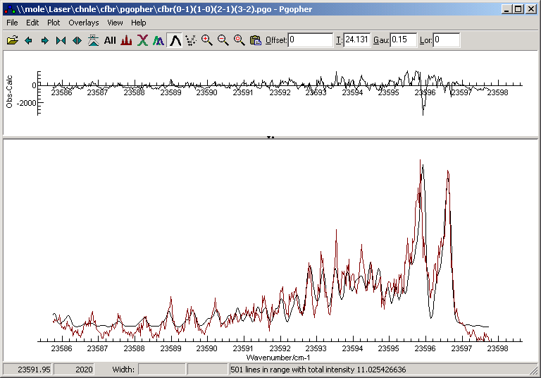
7. Bring up the log window by selecting (View, Log) and choose "Contour" as the fit type in the top left. On pressing the "Fit" button a separate plot showing the obs-calc (difference between the experimental spectrum and the simulation) is shown in the main window (see below for an example), along with the simulation. The log window now shows new values for the floated parameters and their errors, the average error, and a correlation matrix. The error will typically be very large at this point
8. Press the "Fit" button repeatedly, until the average error is as low as possible, and a simulation that roughly matches the experimental spectrum is shown. If you have problems you may have to fix some of the parameters and try manually changing them.
   
9. To further improve the fit, start floating molecular parameters. Floating many parameters simultaneously will often cause the fit to make wild changes in some of the parameters unless the fit is very good. For best results float additional parameters one or two at a time, starting with the most important. The Undo Fit button allows you go back to previous fits, if you find you have gone too far from a reasonable fit. For example, the excited state origin might be the first molecular constant to float (“View”, “Constants”, and click on the “no” next to the constant to change it to yes.). Again, press “Contour fit” repeatedly until the error reaches a minimum, and converges.
10. Other parameters to consider are A or B rotational constants, the linewidth and rotational temperature. Eventually, the simulation should closely resemble the experimental spectrum, and the obs-calc will be much smaller.

The log window will show details of the fit, including estimated standard deviations of the parameters. The standard deviations are calculated using the standard methods for least squares fitting, using derivatives estimated with numerical differences, but experience with contour fitting indicates that the error bars on the parameters are typically too small, and the most reliable estimates of the error are obtained by comparing the results of fits to different data sets.

An estimated error on intensity can be specified for each point to give a weighted fit; the value can be specified by giving an additional column when importing the data, or alternatively given as a function of the position and original intensity - see Calculated Intensity Weight.